Introduction
This blog post and the next are to complement a talk I will give at Infiniteconf. In this series of posts, we will be investigating a learning problem: determining the correct output of an XOR logic gate. To do this, we will build a simple feed-forward deep learning neural network, which will use the backpropagation algorithm to correctly learn from the data provided for this problem. In this first post we will be covering all the details required to set up our deep learning neural network. In the next post, we will then learn how to implement backpropagation, and how the this learning algorithm is used to produce the output matching an XOR gate as closely as possible. To save us some effort moving forward, we will be using numjs to handle numeric operations we need to perform, hence the asterisk in the title.
Before we get to any detail, it’s probably worth reflecting on why deep learning has become such a hot topic in the industry. In a nutshell, deep learning has been shown to outperform more traditional machine learning approaches in a range of applications. In particular, very generic neural networks can be very powerful when it comes to complicated problems such as computer vision: a deep neural network with no specific instruction of its target domain can classify images effectively.
Coming back to the learning problem at a very high level, ultimately we are simply trying to get the correct output for a given input. We are going to follow an approach that falls into the machine learning paradigm known as supervised learning. Initially, we train our network by giving it a set of training data with known inputs and outputs. During this process the network is expected to updated itself so it most closely produces the expected output for the given input - we will cover this in detail in the next blog post. Once we are satisfied with the network’s training progress, we move to a test case. This is where we provide the network with inputs, without telling it upfront what the output should be. Ideally it should be able to match the expected output very closely, provided it has been adequately trained.
I’ve used the word “learning” a few times already, but what do we mean exactly in this context? Simply put, we can think of “learning” as being the process of minimising the network error as it works through the training set. To accomplish this, the network will need to make some adjustments in response to an error calculation which we will cover in part 2. This can equivalently be thought of as a process of finding the correlation or relationship between the training data inputs.
Setup
We better start building our network. Let’s begin by reviewing the example problem we are going to cover, the XOR logic gate. The possible inputs and outputs for XOR can be exhaustively given by the logic table below,
| A | B | A XOR B |
|---|---|---|
| 0 | 0 | 0 |
| 0 | 1 | 1 |
| 1 | 0 | 1 |
| 1 | 1 | 0 |
The XOR gate tells us that our output will only ever be 1 if our inputs are different. This is precisely why XOR has the longform name “exclusive or”, we get a output of 1 if either A or B are 1 but not both.
Given the logic table above, we can say that our input with be an array of length 2, with entries given by A and B respectively. Our output will simply be the integer either 1 or 0. Our training data follows from the logic table, where nj is our import of numjs,
const inputs = nj.array([
    [0, 0],
    [0, 1],
    [1, 0],
    [1, 1]
])

const outputs = nj.array([[0, 1, 1, 0]]).T
What should our network look like to reflect these inputs and outputs? The building block of a neural networks are nodes, these contain activation values that is values our network produces at an arbitrary point in the network. These are basically the “neurons” of our network. The nodes are collected together in layers, such that each layer has common inputs and outputs. Given this information, we will have two layers, an input and an output layer, with the former made of two nodes, and the later just one. Putting this altogether, our network will look something like this,

Where the two input nodes on the left hand side have placeholder values A and B, and our output node has a value O. I’ve also snuck in some numeral values hovering around some arrows connecting our nodes. These are “weights” and they indicate the strength of the relationship between any two nodes - where do they come from? The answer is we randomly pick them. For more sophisticated approaches, you might want to take into account the number of inputs and the underlying problem when selecting weights. We will instead use the simpler approach of choosing from a normal distribution with mean 0 and standard deviation 1. We will also add in another restriction to our weights: they must be between -1 and +1. For our network of two input nodes and one input node, our weights can be generated as follows,
let weightsInputOutput = nj.random([2, 1]).multiply(2).subtract(1)Moving forward, we will often make strange, seemingly arbitrary, choices amongst our parameters. - this is always for the same two reasons. First, we want to keep things as simple as we can for the sake of illustrative purposes. Secondly, we want to make choices to ensure our network learns as quickly as possible, or at least that we don’t make the learning process more difficult than it needs to be.
Together the node values and weights allow us to calculate the value of other nodes in the network, known as the activation. The values of A and B come from our training data, and given our weights we can find the value of O by taking the weighted sum of A and B. The network above would give the value for O in terms of A and B as,
O = 0.4 * A + 0.6 * B
This is true of an arbitrary number of weights and inputs. Instead of working out this sum for each possible output node, we can instead use the dot product which does exactly this sum but across a whole layer at once. Using the dot product, the above equation would become
O = [A, B] • [0.4, 0.6]
We will not do this explicitly in the code sample and instead rely on the implementation provided bynumjs.
At this point we have a working neural network! However, this will not be able to correctly match the XOR output. To do this, we will need to create a deep learning neural network. To walk through the reasons why, I will first introduce a logic gate that could be solved by our present network. The example being the AND gate, with the logic table below,
| A | B | A AND B |
|---|---|---|
| 0 | 0 | 0 |
| 0 | 1 | 0 |
| 1 | 0 | 0 |
| 1 | 1 | 1 |
This logic gate can be correctly mapped to what is known as a linear neural network. The term “linear” used in relation to neural networks refers to both a condition relating to both the input nodes and the expected output, and in either case have important implications for our network. To demonstrate, I’m going to give the AND gate logic table a different representation,
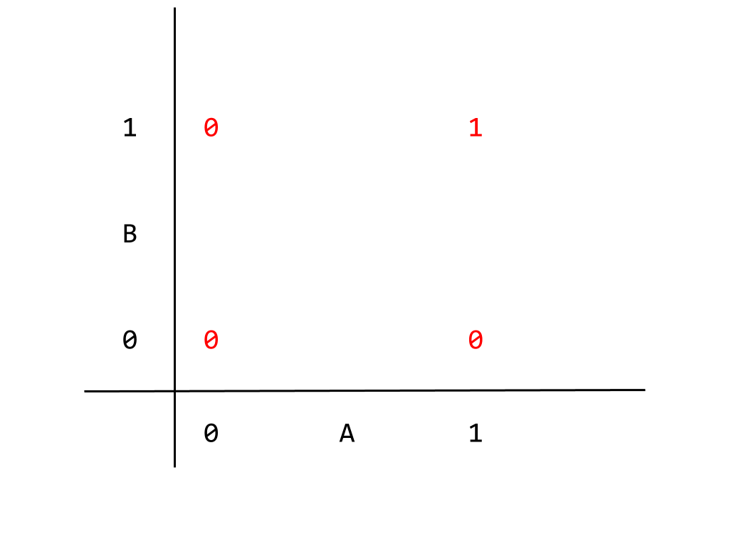
This graph gives the logic table where the inputs correspond to horizontal and vertical axes, and the output appears in red. We can read, for example, the output corresponding to A = B = 1 as being 1 as expected. Given how the output appears in the graph, we can separate the two kinds of output, 0 or 1, with a single linear dividing boundary, given below
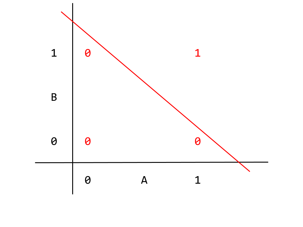
Output that can be divided like this are called “linearly separable”. This is a condition for a problem to be solvable by a linear neural network. Thinking in terms of the inputs instead, given that a linear neural network can produce the correct output implies that exists a correlation between the input nodes that our current neural network correctly captures. It not really important to go into this in any more detail, but bearing this result in mind we can return to the XOR gate. Unlike the AND gate, the XOR gate cannot be solved by a linear neural network precisely because the output is not linearly separable. This point is better illustrated by a graph like the one given for the AND gate,
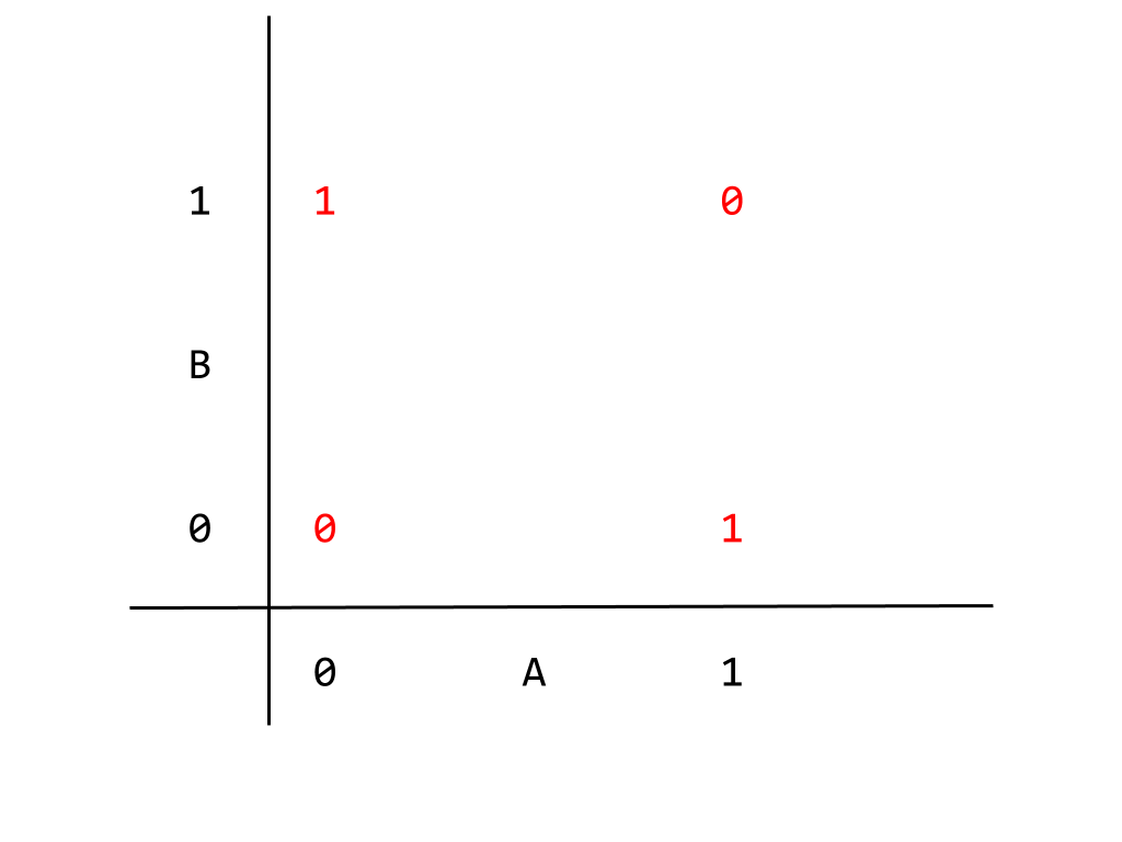
You should be able to eyeball it: we cannot find a single linear dividing boundary between the 0 and 1 outputs.
Moving on from this result, we need to add something else to our network to make it work for an XOR gate: we need to introduce nonlinear behaviour. We need to start by adding other layers of nodes between the input and output layers. This is known as a hidden layer, and is used to create intermediate correlations from our input nodes. In this context, correlation simply means some combination of nodes that produces a new activation. As with other choices we’ve made for our network so far, we are going to go with the simplest choice possible. In this case, we’ll add a single hidden layer with three nodes. Our network now looks like this,
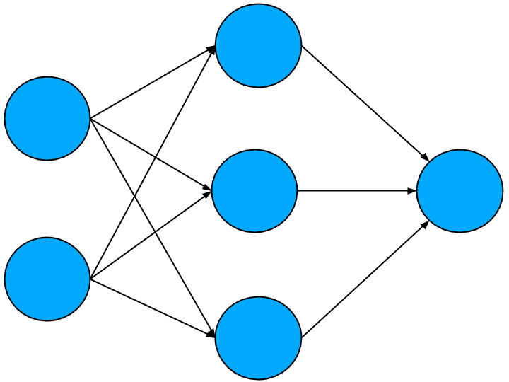
Looks great right? But this is still a linear network. To illustrate, let’s focus on one hidden layer node and the two input nodes and output node it connects to like so,
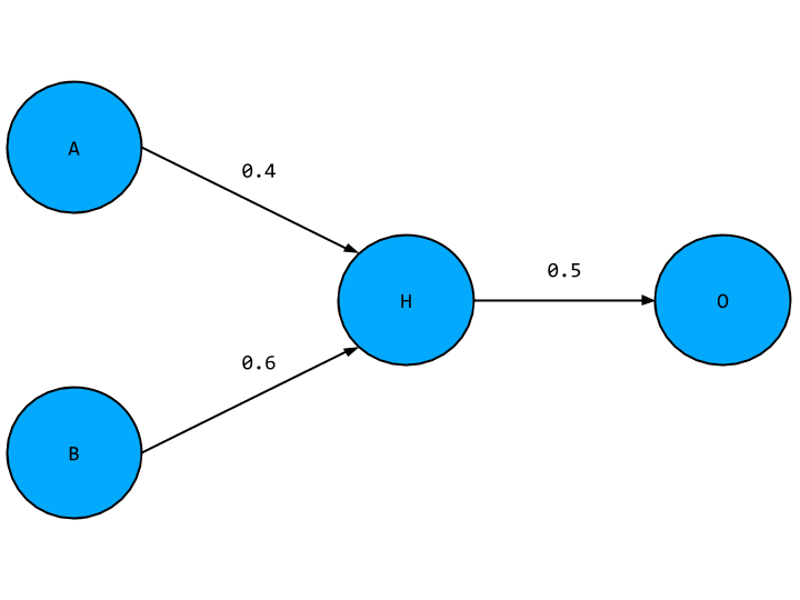
This should look familiar, with the new hidden layer node given a placeholder value H. To find the value of O in terms of A and B we first have to find the value of H. This is simply the weighted sum of A and B,
H = 0.4 * A + 0.6 * B
O is just this expression multiplied by the weight connecting H and O,
O = 0.5 * H = 0.5 * (0.4 * A + 0.6 * B)
And expanding this out,
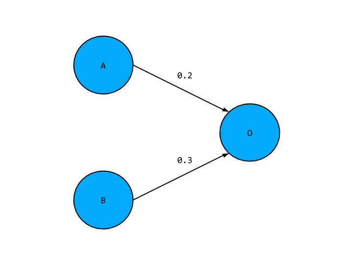
O = 0.2 * A + 0.3 * B
This looks exactly like the output we’d expect from our original linear network, which means the hidden layer node is not adding anything new to our network. In fact our hidden layer as a whole is not giving us any new correlations, so we might as well not have it in this case, and have a network with slightly tweak weights as below,
To move away from a linear network we need to add yet another component: activation functions. This is precisely so that the hidden layer activations is not just some weighted of input nodes, so our network is not simply reducible to a single input and output layer. Activation functions are just mathematical functions that determine whether a hidden layer node turns “on” or “off” for a given input. They fit within the common conceptual picture of neurons in the brain. Like our hidden layer nodes, neurons receive an electrical signal and may signal on or off if this input reaches a certain threshold. The choice of activation ultimately comes down to the kind of problem we are dealing with. The activation function we will be using is known as the “relu” function, which follows the rules:
- If the input value < 0 then return 0
- Otherwise return the original input
Turning to code we get the following,
function relu(x) {
    return iterator(x, x => ((x > 0) * x))
}

function iterator(x, fn) {
    let out = x.slice().tolist()

    for (let i = 0; i < out.length; i++) {
        for (let j = 0; j < out[i].length; j++) {
            out[i][j] = fn(out[i][j])
        }
    }

    return nj.array(out)
}
This has been refactored to use a more functional style, but the basic logic is this same. x => ((x > 0) * x) is the actual relu function as discussed, and the iterator helper function applies this element-by-element on an array of arbitrary size.
That’s a lot of material to cover already, but we now have a deep learning neural network! In the next post we will see how to run input into this network to get output and how to get the network to learn the training set data adequately.
All the best,
Tom