Introduction
In the first post in this series, we created a deep learning neural network so now we have everything in place to actually solve the learning problem we originally introduced: how to create a neural network to correctly match the output of an XOR gate. To do this we need adjust our network weights in response to the output our network produces from the training data. This is what the backpropagation algorithm does. The backpropagation algorithm follows in order,
- Forward propagation: Pass input into our network, and get some output
- Error calculation: Find the error for this output using an error function
- Backward propagation and gradient descent: Work out how this error relates to each weight in our network, and the update the weights in our network, which hopefully improves our output
And iteratively through these three steps until the network converges to the optimal set of weights for the learning problem. This post will take us through a single run of this algorithm.
Forward Propagation
In order to get some output from our network we need to put some input into it, and move this through the network. Forward propagation is a process of finding the activation for a set of inputs and weights layer by layer. This is simply the dot product of the inputs with the weights,
activation = nodes • weights
For the hidden layer we have the additional step of plugging this result through the activation function,
activation = relu(nodes • weights)
For our network, taking a single hidden layer node, we have,
- Input layer values A, B, just comes from the training data
- Hidden layer node,
H = relu([A, B] • [w_ih_A, w_ih_B]) - Output node,
O = H • w_ho = relu([A, B] • [w_ih_A, w_ih_B]^T) * w_ho
This is exactly the same process we would use to find out the value for O, our output value, for all nodes and weights. The code for this step is as follows,
for (let iteration = 0; iteration < 60; iteration++) {
    for (let i = 0; i < inputs.shape[0]; i++) {
        let inputLayer = inputs.slice([i, i + 1])
        let hiddenLayer = relu(nj.dot(inputLayer, inputHiddenWeights))
        let outputLayer = nj.dot(hiddenLayer, hiddenOutputWeights)
    }
}
As can be seen in the code sample, the process is run over an arbitrary number of iterations for the sake of illustration.
Error Calculation
From the previous step, we got some output from the network - but how do we know if this is any good? We need to be able to find how closely this matches the training data output values, or in other words, find the error that our network output produces. After all, we want our to learn the training data and as we said in part 1, learning is just a process of error minimisation. To quantify the network error we are going to be using something called the squared error,
error = (output - target) ** 2
Our error will only ever be a value greater than or equal to zero, where the lower the value the better our network is doing. Think about it this way, if I shoot an arrow at a target, I don’t care if I’m above/below or to the left/right of the target - just by how much I missed.
You may still have the lingering question as to why we introduce this “extra” quantity of error, when we are really jsut worried about the network weights. It is simply that the error is very easy to track and see improvements in the network. Think of it this way, if the error increases we know the network is doing worse, and conversely if it decreases. If instead we just tracked the weights, we wouldn’t necessarily know what a given change in the weights meant for our network’s performance. Furthermore, as we’ll see in the next section an error function like the squared error is guaranteed to converge - at least for some choice of parameters. This implies that we can achieve the optimal set of weights for the learning problem using this approach. The
for (let iteration = 0; iteration < 60; iteration++) {
    let error = 0

    for (let i = 0; i < inputs.shape[0]; i++) {
        //  Forward propagation step ...

        error = nj.add(error, nj.sum(nj.power((nj.subtract(outputLayer, outputs.slice([i, i + 1]))), 2)))

    }

}
Backward Propagation and Gradient Descent
At this point we have some output from our network and an error. So we know how well our network is doing, but how do we improve this error? It turns out that we can only change the weights. We have at our disposal the weights and the training data. However, we don’t want to change the training data as we want this to be an accurate reflection of the problem at hand. If we tweak the training data to get the network to train more efficiently we are only selling ourselves short: Once we move to the test case, the network would likely underperform as it not learnt data matching the learning problem. The takeaway is that we should only think about changing the weights during this process.
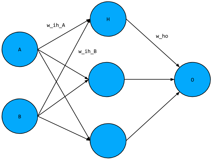
During this step, we work backwards through the network and determine how much to change each weight by finding how the error function changes with respect to each weight. The actual process of updating each weight is gradient descent’s responsibility. To illustrate how this is done, we will look at a single weight between each layer, see the network diagram below,
where as before we have placeholder variables for each node value as well as for the weights, where w_ho is the weight connecting the hidden layer node to the output not, and w_ih is the weight connecting the input node to the hidden layer node.
Firstly let’s determine how the error function changes in response to w_ho. We know what the error function looks like,
error = (output - target) ** 2
but we need to get this in terms of w_ho. To do this, recall that the output, O for a single node is given as the multiplication between the activation of the node in the previous layer with the weight connecting the two,
output = activation * weight
For this example the activation is given by H (we don’t care where this came from as we’ll justify in a bit), and the weight is w_ho, so plugging these into the above equation we get,
O = H * w_ho
With this expression for the output, O, we can plug this into our error function to get,
error = ((H * w_ho) - target) ** 2
giving us the error function in terms of w_ho. We can make a further simplification by reminding ourselves where H and target come from. The target value comes from our training data and so as discussed above is not something we are free to vary. The activation, H, is also a constant during this process as we are not feeding in new input values during this step of the backpropagation algorithm. Altogether that means that the only variable we have to play with is the weight, so the error function is simply the square of w_ho,
error ~ w_ho ** 2
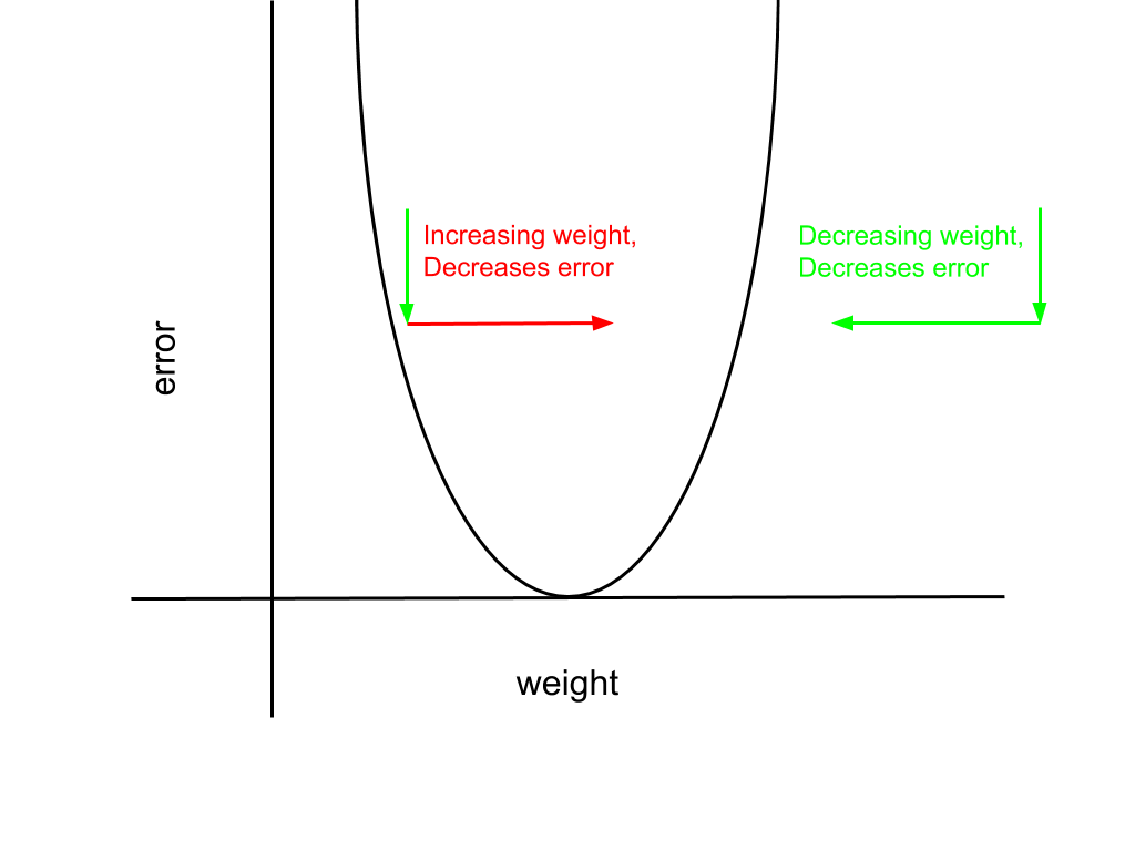
This is just a parabola, which has a simple graph,
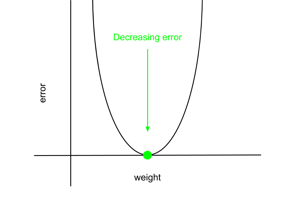
Indicated on the graph as a green point is the minimum of the error function, where the error is zero, which is the point we want to reach. The corresponding weight that minimises the error is the goal weight. To reach the minimum from an arbitrary point on the parabola, we need to ask ourselves: what is the change in the error for a given change in the weight value? The approach that gradient descent takes is greedy, it just takes the change in the weight that changes the error most. This is just a verbose way of saying we need to find the derivative of the error function with respect to a given weight to determine the weight update. Indicated below, the derivative is the slope of the line at the point given by the dashed lines.
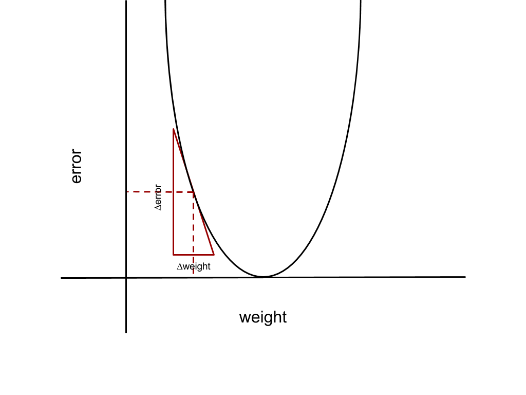
In general, the derivative gives us the relationship between a set of variables, in our case that is how the change in the the weight, ∆weight, relates to the change in the error, ∆error, which is just the product of the derivative with the change in weight,
∆error = derivative * ∆weight
The derivative is calculated from the expression for the error function given above. I’ll just give it to you, but it is quite easy to find for yourselves,
derivative ~ H * (O - target)
We now know how much to update the weight, which is just the derivative, but do we add or subtract this amount from the current weight value? Going back the parabola that gives the relationship between the weight and the error we find that we add or subtract this update depending as to which side of the goal weight we find ourselves. If we are to the left of the goal weight, the derivative is always negative, as the graph is sloping downwards. However, in order to decrease the error, we need to increase the weight to move towards the goal weight. This means we should take the negative of the derivative as our weight update, so this is a positive number. The converse argument holds if we start to the right of the goal weight: The derivative is positive, but we need to decrease the weight to decrease the error. Both scenarios are illustrated below.
Putting this all together, the weight update for weights connecting the hidden layer nodes and output nodes, like w_ho, is given by,
weight -= activation * (output - target)If we were to repeat this process for many iterations, we simply continue until we converge to this goal weight. A consequence of the error function we’ve chosen for our network, a parabola, means that the goal weight is in fact a global minimum, meaning that as long as we can guarantee convergence we will achieve the optimal weight for the learning problem. This is something we’ll return to later.
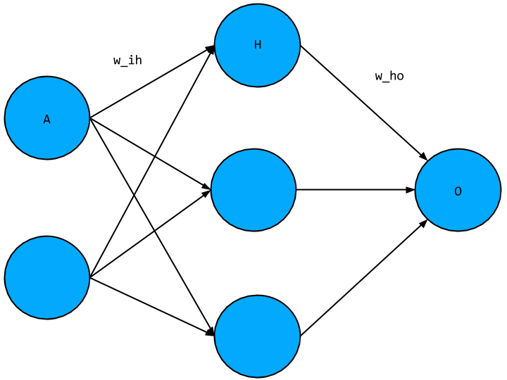
Now that we know how to update the weights between the hidden and output layer, we can use the same process to update the weights connecting the input and hidden layer. Going back to the network diagram,
We need to find the change in the error function with respect to w_ih. This is the same process as before but complicated by the activation function. We need to express the error function as a function of w_ih. To do this we need to first express the output O in terms of H and w_ho, which as before is just the product,
O = H * w_ho
This time around however, H is not fixed for us as it comes from w_ih which we are varying. This means we need to express H in terms of A and w_ih. H is a hidden layer node, so the activation H is given as,
H = relu(A * w_ih)
now plugging this into our previous equation for O,
O = relu(A * w_ih) * w_ho
and finally we plug this into the error function to express the error function in terms of w_ih,
error = (relu(A * w_ih) * w_ho - target) ** 2
Having expressed the error function in terms of w_ih we need to find the derivative of the error function with respect to w_ih, which will give us the size of the weight update. This is more complicated than before as we need to take the derivative of the activation function, relu, into account as well. As before, I will skip over the details and just give the result,
derivative ~ (O - target) * reluDeriv(A * w_ih) * A * w_ho
This expression looks pretty dense, especially as we have factors of w_ho and reluDeriv which we haven’t seen in the previous weight update. There is however a fairly intuitive explanation for their presence, which relates to the key aspect of the backpropagation process: we are going back through the network and attributing the final error to each of the weights. To illustrate this point, take for example the limit of w_ho, that is as it approaches zero. If w_ho were zero, then that would imply that the activation H, and any weight that produced H, couldn’t have contributed to the final error - so we shouldn’t update w_ih in this iteration. A similar reasoning applies to reluDeriv. In part 1, we saw that relu produced an activation equal to or greater than zero, which means either the activation did or didn’t contribute to the final error. reluDeriv captures this intuition, which is given by the following function,
reluDeriv = (x) => (x > 0 ? 1 : 0)This returns 1 if and only if the A * w_ih is greater than zero, otherwise it returns 0, where a returned value of 1 means the activation did contribute to the final error and 0 if it didn’t.
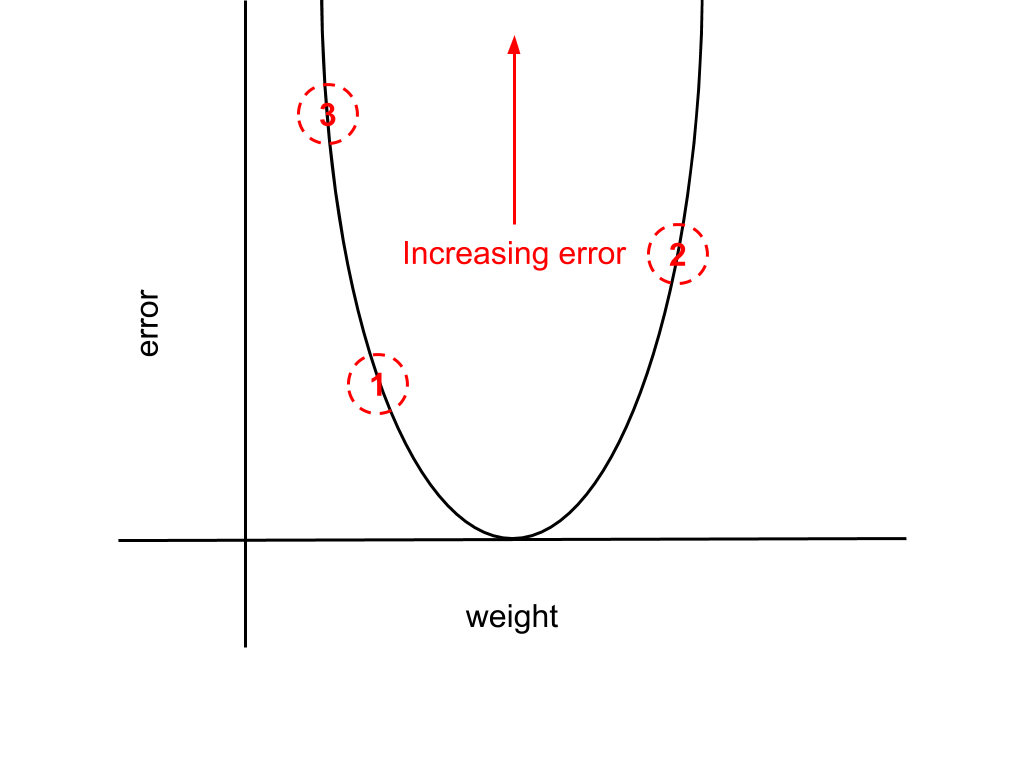
Altogether, these derivatives give us all the weight updates we need for our network. But do these converge to a set of goal weights? Above, I’ve teased that this should be possible, but there is a chance that convergence may not occur. This is because all the weight updates we have scale with the activation value, meaning that there is a risk of divergence if the activation grows too large (these are not normalised). For instance, the derivative the error function with respect to w_ho was found to be,
derivative ~ activation * (output - target)
The diagram below illustrates this point. Iteration-by-iteration the network error will increase as our weight moves increasingly further from the minimum, alternating either side of the goal weight.
The fix for this is quite simple: we just introduce a new multiplicative factor to scale the derivative. This factor is termed the “learning rate” and usually referred to as “alpha”. Adding this to the derivative just given with respect to w_ho we have,
weight -= alpha * activation * (output - target)
There are some important considerations to make when choosing alpha, as it has a direct impact on the rate of convergence of the weights - this is by no means a trivial problem in general. However, for our purposes it will be ok to just choose a fixed number between 0 and 1. Putting this all together, our code for backpropagation and gradient descent is,
const alpha = 0.2

//  Other parameters ...

for (let iteration = 0; iteration < 1; iteration++) {
    let error = 0

    for (let i = 0; i < inputs.shape[0]; i++) {
        //  Forward propagation step ...

        //  Error calculation step ...

        let outputLayerDelta = nj.subtract(outputLayer, outputs.slice([i, i + 1]))
        let hiddenLayerDelta = nj.multiply(outputLayerDelta.dot(hiddenOutputWeights.T), reluDeriv(hiddenLayer))
        hiddenOutputWeights = nj.subtract(hiddenOutputWeights, hiddenLayer.T.dot(outputLayerDelta).multiply(alpha))
        inputHiddenWeights = nj.subtract(inputHiddenWeights, inputLayer.T.dot(hiddenLayerDelta).multiply(alpha))
    }

}
Recap
We’ve covered a lot of material in these two blog posts. Taking it from the top, we chose a learning problem, the XOR logic gate, and matched it to a deep learning neural network. We were able to justify our choices for the network such as the error function and other parameters. Having done all this we worked through a single iteration of the backpropagation algorithm to demonstrate how we would update our network weights by adjusting the weights. Hopefully, this goes someway to demonstrate how deep learning neural networks work from the ground up, and how the choice of learning problem influences the choices we make.
Coming to the end of this series we have a complete network, which will be able to train correctly for the XOR learning problem. The full code sample is available as a gist. If you have any other questions please get in touch.
References
My main resources for these blog post were “Grokking Deep Learning” by Andrew Trask, “Machine Learning Study Group” notes by Nikolay Manchev, and “Neural Networks and Deep Learning” by Michael Nielsen.
All the best,
Tom