Neural Networks from Scratch* Part 2: Backpropagation
Introduction
In the first post in this series, we created a deep learning neural network so now we have everything in place to actually solve the learning problem we originally introduced: how to create a neural network to correctly match the output of an XOR gate. To do this we need adjust our network weights in response to the output our network produces from the training data. This is what the backpropagation algorithm does. The backpropagation algorithm follows in order,
- Forward propagation: Pass input into our network, and get some output
- Error calculation: Find the error for this output using an error function
- Backward propagation and gradient descent: Work out how this error relates to each weight in our network, and the update the weights in our network, which hopefully improves our output
And iteratively through these three steps until the network converges to the optimal set of weights for the learning problem. This post will take us through a single run of this algorithm.
Forward Propagation
In order to get some output from our network we need to put some input into it, and move this through the network. Forward propagation is a process of finding the activation for a set of inputs and weights layer by layer. This is simply the dot product of the inputs with the weights,
activation = nodes • weights
For the hidden layer we have the additional step of plugging this result through the activation function,
activation = relu(nodes • weights)
For our network, taking a single hidden layer node, we have,
- Input layer values A, B, just comes from the training data
- Hidden layer node,
H = relu([A, B] • [w_ih_A, w_ih_B]) - Output node,
O = H • w_ho = relu([A, B] • [w_ih_A, w_ih_B]^T) * w_ho
This is exactly the same process we would use to find out the value for O, our output value, for all nodes and weights. The code for this step is as follows,
for (let iteration = 0; iteration < 60; iteration++) {
    for (let i = 0; i < inputs.shape[0]; i++) {
        let inputLayer = inputs.slice([i, i + 1])
        let hiddenLayer = relu(nj.dot(inputLayer, inputHiddenWeights))
        let outputLayer = nj.dot(hiddenLayer, hiddenOutputWeights)
    }
}
As can be seen in the code sample, the process is run over an arbitrary number of iterations for the sake of illustration.
Error Calculation
From the previous step, we got some output from the network - but how do we know if this is any good? We need to be able to find how closely this matches the training data output values, or in other words, find the error that our network output produces. After all, we want our to learn the training data and as we said in part 1, learning is just a process of error minimisation. To quantify the network error we are going to be using something called the squared error,
error = (output - target) ** 2
Our error will only ever be a value greater than or equal to zero, where the lower the value the better our network is doing. Think about it this way, if I shoot an arrow at a target, I don’t care if I’m above/below or to the left/right of the target - just by how much I missed.
You may still have the lingering question as to why we introduce this “extra” quantity of error, when we are really jsut worried about the network weights. It is simply that the error is very easy to track and see improvements in the network. Think of it this way, if the error increases we know the network is doing worse, and conversely if it decreases. If instead we just tracked the weights, we wouldn’t necessarily know what a given change in the weights meant for our network’s performance. Furthermore, as we’ll see in the next section an error function like the squared error is guaranteed to converge - at least for some choice of parameters. This implies that we can achieve the optimal set of weights for the learning problem using this approach. The
for (let iteration = 0; iteration < 60; iteration++) {
    let error = 0

    for (let i = 0; i < inputs.shape[0]; i++) {
        //  Forward propagation step ...

        error = nj.add(error, nj.sum(nj.power((nj.subtract(outputLayer, outputs.slice([i, i + 1]))), 2)))

    }

}
Backward Propagation and Gradient Descent
At this point we have some output from our network and an error. So we know how well our network is doing, but how do we improve this error? It turns out that we can only change the weights. We have at our disposal the weights and the training data. However, we don’t want to change the training data as we want this to be an accurate reflection of the problem at hand. If we tweak the training data to get the network to train more efficiently we are only selling ourselves short: Once we move to the test case, the network would likely underperform as it not learnt data matching the learning problem. The takeaway is that we should only think about changing the weights during this process.
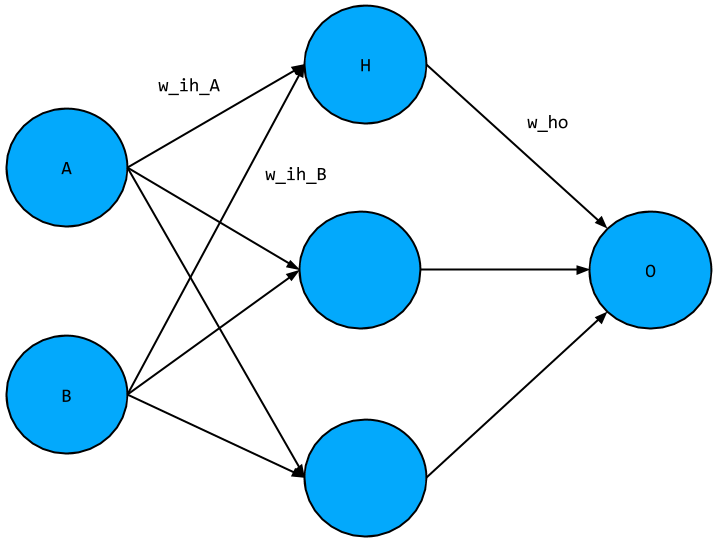
During this step, we work backwards through the network and determine how much to change each weight by finding how the error function changes with respect to each weight. The actual process of updating each weight is gradient descent’s responsibility. To illustrate how this is done, we will look at a single weight between each layer, see the network diagram below,

where as before we have placeholder variables for each node value as well as for the weights, where w_ho is the weight connecting the hidden layer node to the output not, and w_ih is the weight connecting the input node to the hidden layer node.
Firstly let’s determine how the error function changes in response to w_ho. We know what the error function looks like,
error = (output - target) ** 2
but we need to get this in terms of w_ho. To do this, recall that the output, O for a single node is given as the multiplication between the activation of the node in the previous layer with the weight connecting the two,
output = activation * weight
For this example the activation is given by H (we don’t care where this came from as we’ll justify in a bit), and the weight is w_ho, so plugging these into the above equation we get,
O = H * w_ho
With this expression for the output, O, we can plug this into our error function to get,
error = ((H * w_ho) - target) ** 2
giving us the error function in terms of w_ho. We can make a further simplification by reminding ourselves where H and target come from. The target value comes from our training data and so as discussed above is not something we are free to vary. The activation, H, is also a constant during this process as we are not feeding in new input values during this step of the backpropagation algorithm. Altogether that means that the only variable we have to play with is the weight, so the error function is simply the square of w_ho,
error ~ w_ho ** 2
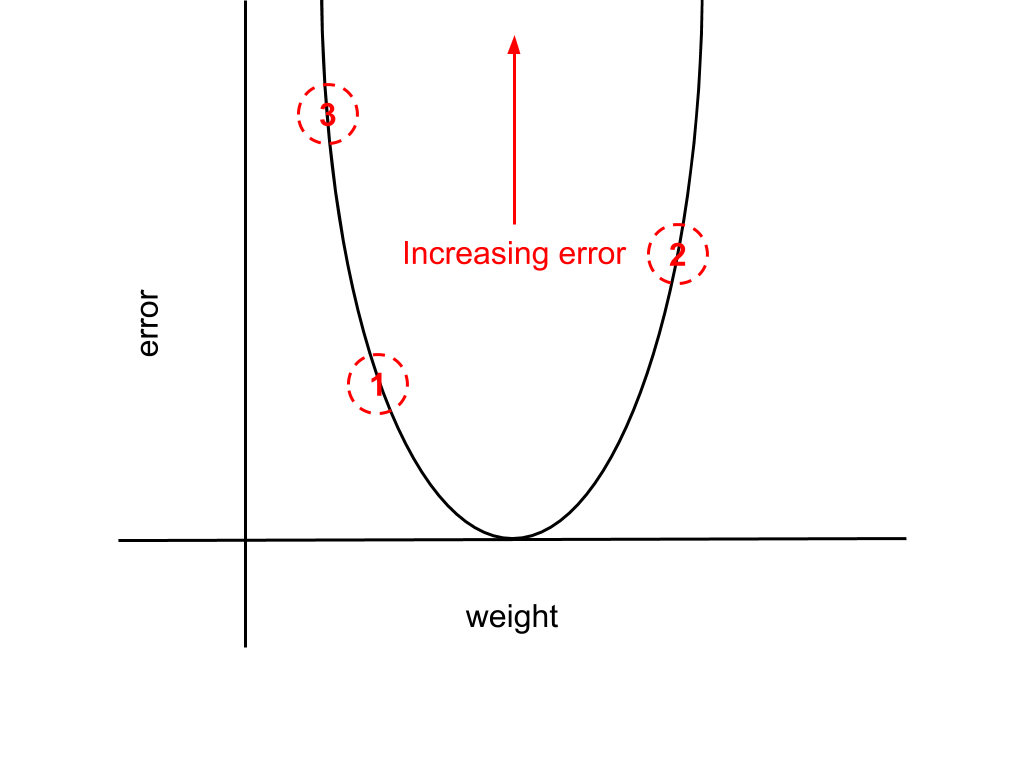
This is just a parabola, which has a simple graph,
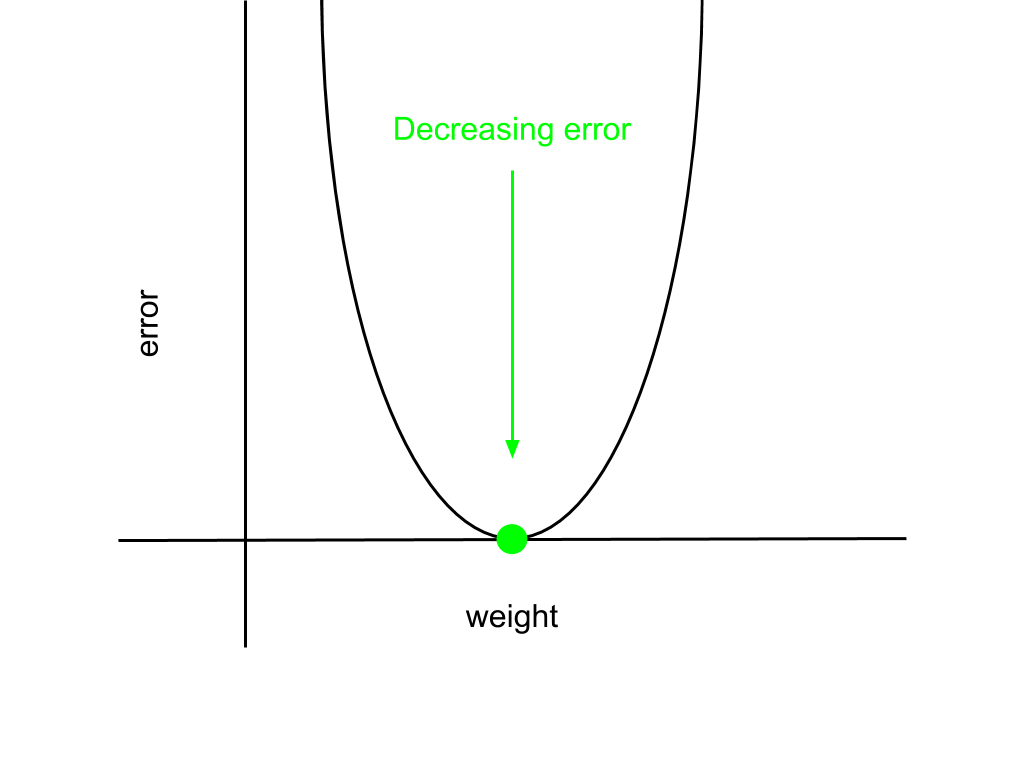
Indicated on the graph as a green point is the minimum of the error function, where the error is zero, which is the point we want to reach. The corresponding weight that minimises the error is the goal weight. To reach the minimum from an arbitrary point on the parabola, we need to ask ourselves: what is the change in the error for a given change in the weight value? The approach that gradient descent takes is greedy, it just takes the change in the weight that changes the error most. This is just a verbose way of saying we need to find the derivative of the error function with respect to a given weight to determine the weight update. Indicated below, the derivative is the slope of the line at the point given by the dashed lines.
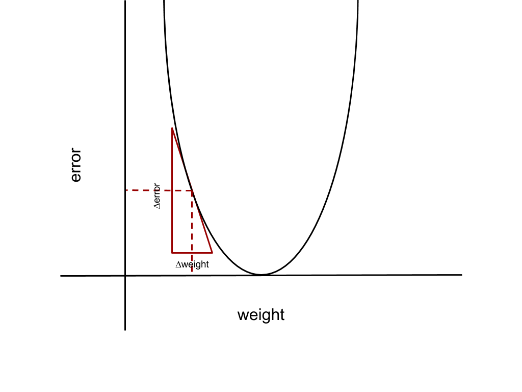
In general, the derivative gives us the relationship between a set of variables, in our case that is how the change in the the weight, ∆weight, relates to the change in the error, ∆error, which is just the product of the derivative with the change in weight,
∆error = derivative * ∆weight
The derivative is calculated from the expression for the error function given above. I’ll just give it to you, but it is quite easy to find for yourselves,
derivative ~ H * (O - target)
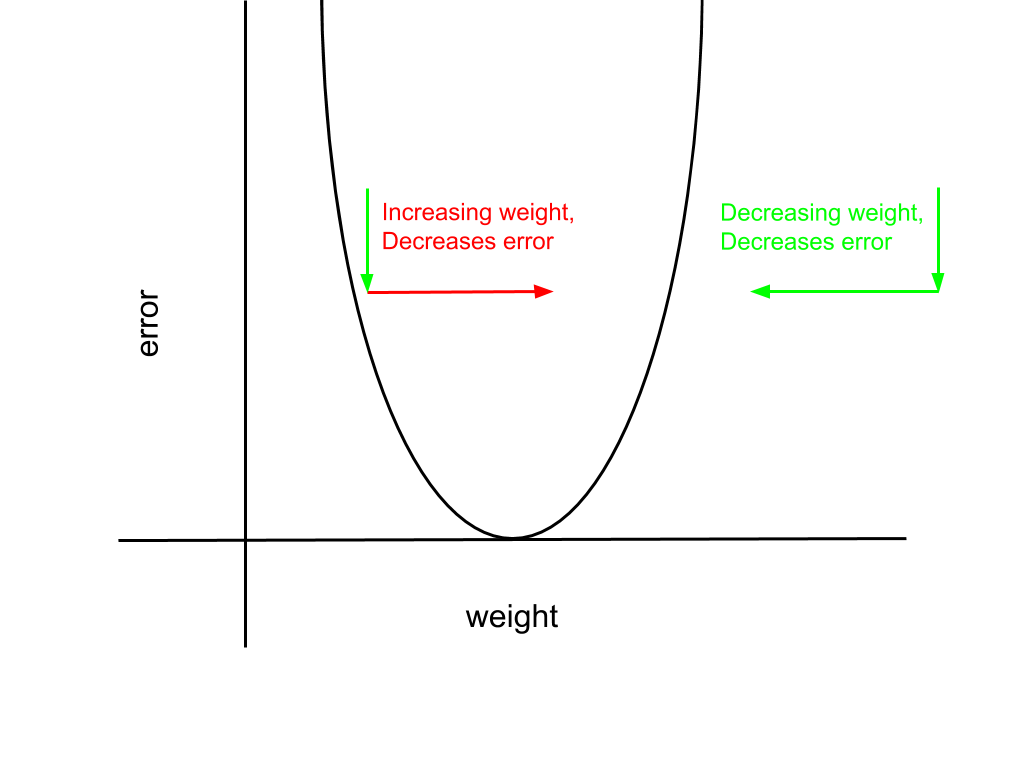
We now know how much to update the weight, which is just the derivative, but do we add or subtract this amount from the current weight value? Going back the parabola that gives the relationship between the weight and the error we find that we add or subtract this update depending as to which side of the goal weight we find ourselves. If we are to the left of the goal weight, the derivative is always negative, as the graph is sloping downwards. However, in order to decrease the error, we need to increase the weight to move towards the goal weight. This means we should take the negative of the derivative as our weight update, so this is a positive number. The converse argument holds if we start to the right of the goal weight: The derivative is positive, but we need to decrease the weight to decrease the error. Both scenarios are illustrated below.
Putting this all together, the weight update for weights connecting the hidden layer nodes and output nodes, like w_ho, is given by,
weight -= activation * (output - target)If we were to repeat this process for many iterations, we simply continue until we converge to this goal weight. A consequence of the error function we’ve chosen for our network, a parabola, means that the goal weight is in fact a global minimum, meaning that as long as we can guarantee convergence we will achieve the optimal weight for the learning problem. This is something we’ll return to later.
Now that we know how to update the weights between the hidden and output layer, we can use the same process to update the weights connecting the input and hidden layer. Going back to the network diagram,
We need to find the change in the error function with respect to w_ih. This is the same process as before but complicated by the activation function. We need to express the error function as a function of w_ih. To do this we need to first express the output O in terms of H and w_ho, which as before is just the product,
O = H * w_ho
This time around however, H is not fixed for us as it comes from w_ih which we are varying. This means we need to express H in terms of A and w_ih. H is a hidden layer node, so the activation H is given as,
H = relu(A * w_ih)
now plugging this into our previous equation for O,
O = relu(A * w_ih) * w_ho
and finally we plug this into the error function to express the error function in terms of w_ih,
error = (relu(A * w_ih) * w_ho - target) ** 2
Having expressed the error function in terms of w_ih we need to find the derivative of the error function with respect to w_ih, which will give us the size of the weight update. This is more complicated than before as we need to take the derivative of the activation function, relu, into account as well. As before, I will skip over the details and just give the result,
derivative ~ (O - target) * reluDeriv(A * w_ih) * A * w_ho
This expression looks pretty dense, especially as we have factors of w_ho and reluDeriv which we haven’t seen in the previous weight update. There is however a fairly intuitive explanation for their presence, which relates to the key aspect of the backpropagation process: we are going back through the network and attributing the final error to each of the weights. To illustrate this point, take for example the limit of w_ho, that is as it approaches zero. If w_ho were zero, then that would imply that the activation H, and any weight that produced H, couldn’t have contributed to the final error - so we shouldn’t update w_ih in this iteration. A similar reasoning applies to reluDeriv. In part 1, we saw that relu produced an activation equal to or greater than zero, which means either the activation did or didn’t contribute to the final error. reluDeriv captures this intuition, which is given by the following function,
reluDeriv = (x) => (x > 0 ? 1 : 0)This returns 1 if and only if the A * w_ih is greater than zero, otherwise it returns 0, where a returned value of 1 means the activation did contribute to the final error and 0 if it didn’t.
Altogether, these derivatives give us all the weight updates we need for our network. But do these converge to a set of goal weights? Above, I’ve teased that this should be possible, but there is a chance that convergence may not occur. This is because all the weight updates we have scale with the activation value, meaning that there is a risk of divergence if the activation grows too large (these are not normalised). For instance, the derivative the error function with respect to w_ho was found to be,
derivative ~ activation * (output - target)
The diagram below illustrates this point. Iteration-by-iteration the network error will increase as our weight moves increasingly further from the minimum, alternating either side of the goal weight.
The fix for this is quite simple: we just introduce a new multiplicative factor to scale the derivative. This factor is termed the “learning rate” and usually referred to as “alpha”. Adding this to the derivative just given with respect to w_ho we have,
weight -= alpha * activation * (output - target)
There are some important considerations to make when choosing alpha, as it has a direct impact on the rate of convergence of the weights - this is by no means a trivial problem in general. However, for our purposes it will be ok to just choose a fixed number between 0 and 1. Putting this all together, our code for backpropagation and gradient descent is,
const alpha = 0.2

//  Other parameters ...

for (let iteration = 0; iteration < 1; iteration++) {
    let error = 0

    for (let i = 0; i < inputs.shape[0]; i++) {
        //  Forward propagation step ...

        //  Error calculation step ...

        let outputLayerDelta = nj.subtract(outputLayer, outputs.slice([i, i + 1]))
        let hiddenLayerDelta = nj.multiply(outputLayerDelta.dot(hiddenOutputWeights.T), reluDeriv(hiddenLayer))
        hiddenOutputWeights = nj.subtract(hiddenOutputWeights, hiddenLayer.T.dot(outputLayerDelta).multiply(alpha))
        inputHiddenWeights = nj.subtract(inputHiddenWeights, inputLayer.T.dot(hiddenLayerDelta).multiply(alpha))
    }

}
Recap
We’ve covered a lot of material in these two blog posts. Taking it from the top, we chose a learning problem, the XOR logic gate, and matched it to a deep learning neural network. We were able to justify our choices for the network such as the error function and other parameters. Having done all this we worked through a single iteration of the backpropagation algorithm to demonstrate how we would update our network weights by adjusting the weights. Hopefully, this goes someway to demonstrate how deep learning neural networks work from the ground up, and how the choice of learning problem influences the choices we make.
Coming to the end of this series we have a complete network, which will be able to train correctly for the XOR learning problem. The full code sample is available as a gist. If you have any other questions please get in touch.
References
My main resources for these blog post were “Grokking Deep Learning” by Andrew Trask, “Machine Learning Study Group” notes by Nikolay Manchev, and “Neural Networks and Deep Learning” by Michael Nielsen.
All the best,
Tom
Neural Networks from Scratch* Part 1: Building the Network
Introduction
This blog post and the next are to complement a talk I will give at Infiniteconf. In this series of posts, we will be investigating a learning problem: determining the correct output of an XOR logic gate. To do this, we will build a simple feed-forward deep learning neural network, which will use the backpropagation algorithm to correctly learn from the data provided for this problem. In this first post we will be covering all the details required to set up our deep learning neural network. In the next post, we will then learn how to implement backpropagation, and how the this learning algorithm is used to produce the output matching an XOR gate as closely as possible. To save us some effort moving forward, we will be using numjs to handle numeric operations we need to perform, hence the asterisk in the title.
Before we get to any detail, it’s probably worth reflecting on why deep learning has become such a hot topic in the industry. In a nutshell, deep learning has been shown to outperform more traditional machine learning approaches in a range of applications. In particular, very generic neural networks can be very powerful when it comes to complicated problems such as computer vision: a deep neural network with no specific instruction of its target domain can classify images effectively.
Coming back to the learning problem at a very high level, ultimately we are simply trying to get the correct output for a given input. We are going to follow an approach that falls into the machine learning paradigm known as supervised learning. Initially, we train our network by giving it a set of training data with known inputs and outputs. During this process the network is expected to updated itself so it most closely produces the expected output for the given input - we will cover this in detail in the next blog post. Once we are satisfied with the network’s training progress, we move to a test case. This is where we provide the network with inputs, without telling it upfront what the output should be. Ideally it should be able to match the expected output very closely, provided it has been adequately trained.
I’ve used the word “learning” a few times already, but what do we mean exactly in this context? Simply put, we can think of “learning” as being the process of minimising the network error as it works through the training set. To accomplish this, the network will need to make some adjustments in response to an error calculation which we will cover in part 2. This can equivalently be thought of as a process of finding the correlation or relationship between the training data inputs.
Setup
We better start building our network. Let’s begin by reviewing the example problem we are going to cover, the XOR logic gate. The possible inputs and outputs for XOR can be exhaustively given by the logic table below,
| A | B | A XOR B |
|---|---|---|
| 0 | 0 | 0 |
| 0 | 1 | 1 |
| 1 | 0 | 1 |
| 1 | 1 | 0 |
The XOR gate tells us that our output will only ever be 1 if our inputs are different. This is precisely why XOR has the longform name “exclusive or”, we get a output of 1 if either A or B are 1 but not both.
Given the logic table above, we can say that our input with be an array of length 2, with entries given by A and B respectively. Our output will simply be the integer either 1 or 0. Our training data follows from the logic table, where nj is our import of numjs,
const inputs = nj.array([
    [0, 0],
    [0, 1],
    [1, 0],
    [1, 1]
])

const outputs = nj.array([[0, 1, 1, 0]]).T
What should our network look like to reflect these inputs and outputs? The building block of a neural networks are nodes, these contain activation values that is values our network produces at an arbitrary point in the network. These are basically the “neurons” of our network. The nodes are collected together in layers, such that each layer has common inputs and outputs. Given this information, we will have two layers, an input and an output layer, with the former made of two nodes, and the later just one. Putting this altogether, our network will look something like this,

Where the two input nodes on the left hand side have placeholder values A and B, and our output node has a value O. I’ve also snuck in some numeral values hovering around some arrows connecting our nodes. These are “weights” and they indicate the strength of the relationship between any two nodes - where do they come from? The answer is we randomly pick them. For more sophisticated approaches, you might want to take into account the number of inputs and the underlying problem when selecting weights. We will instead use the simpler approach of choosing from a normal distribution with mean 0 and standard deviation 1. We will also add in another restriction to our weights: they must be between -1 and +1. For our network of two input nodes and one input node, our weights can be generated as follows,
let weightsInputOutput = nj.random([2, 1]).multiply(2).subtract(1)Moving forward, we will often make strange, seemingly arbitrary, choices amongst our parameters. - this is always for the same two reasons. First, we want to keep things as simple as we can for the sake of illustrative purposes. Secondly, we want to make choices to ensure our network learns as quickly as possible, or at least that we don’t make the learning process more difficult than it needs to be.
Together the node values and weights allow us to calculate the value of other nodes in the network, known as the activation. The values of A and B come from our training data, and given our weights we can find the value of O by taking the weighted sum of A and B. The network above would give the value for O in terms of A and B as,
O = 0.4 * A + 0.6 * B
This is true of an arbitrary number of weights and inputs. Instead of working out this sum for each possible output node, we can instead use the dot product which does exactly this sum but across a whole layer at once. Using the dot product, the above equation would become
O = [A, B] • [0.4, 0.6]
We will not do this explicitly in the code sample and instead rely on the implementation provided bynumjs.
At this point we have a working neural network! However, this will not be able to correctly match the XOR output. To do this, we will need to create a deep learning neural network. To walk through the reasons why, I will first introduce a logic gate that could be solved by our present network. The example being the AND gate, with the logic table below,
| A | B | A AND B |
|---|---|---|
| 0 | 0 | 0 |
| 0 | 1 | 0 |
| 1 | 0 | 0 |
| 1 | 1 | 1 |
This logic gate can be correctly mapped to what is known as a linear neural network. The term “linear” used in relation to neural networks refers to both a condition relating to both the input nodes and the expected output, and in either case have important implications for our network. To demonstrate, I’m going to give the AND gate logic table a different representation,
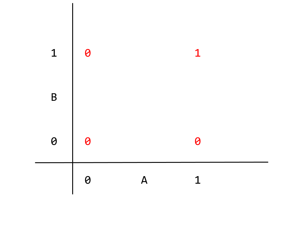
This graph gives the logic table where the inputs correspond to horizontal and vertical axes, and the output appears in red. We can read, for example, the output corresponding to A = B = 1 as being 1 as expected. Given how the output appears in the graph, we can separate the two kinds of output, 0 or 1, with a single linear dividing boundary, given below
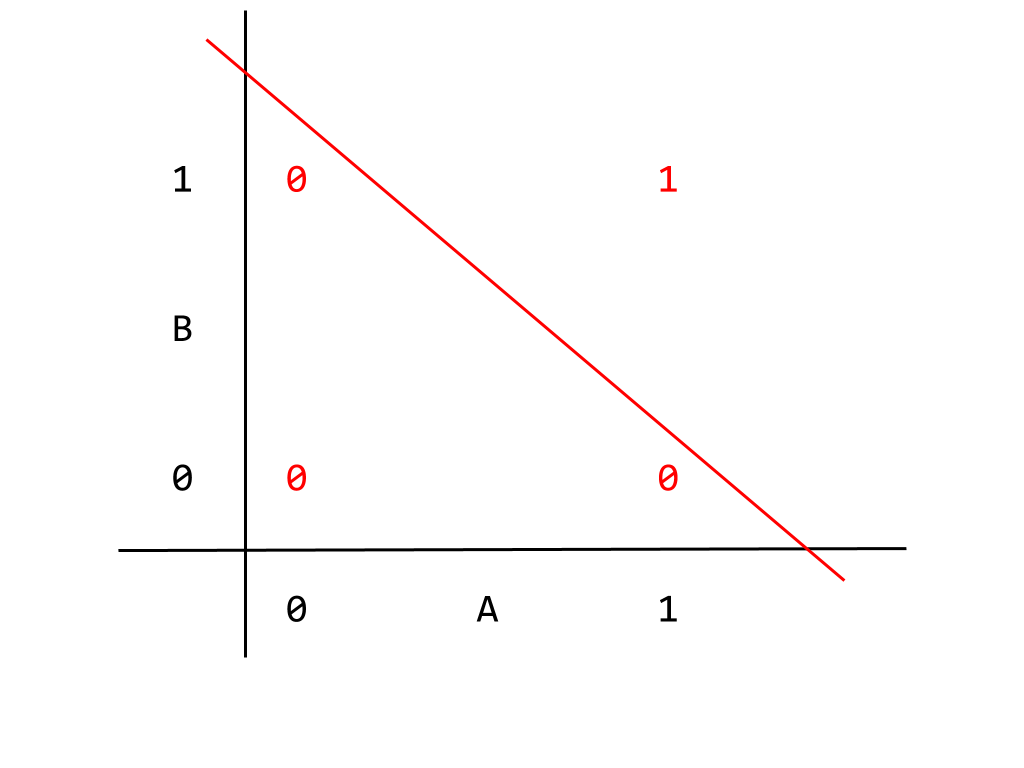
Output that can be divided like this are called “linearly separable”. This is a condition for a problem to be solvable by a linear neural network. Thinking in terms of the inputs instead, given that a linear neural network can produce the correct output implies that exists a correlation between the input nodes that our current neural network correctly captures. It not really important to go into this in any more detail, but bearing this result in mind we can return to the XOR gate. Unlike the AND gate, the XOR gate cannot be solved by a linear neural network precisely because the output is not linearly separable. This point is better illustrated by a graph like the one given for the AND gate,
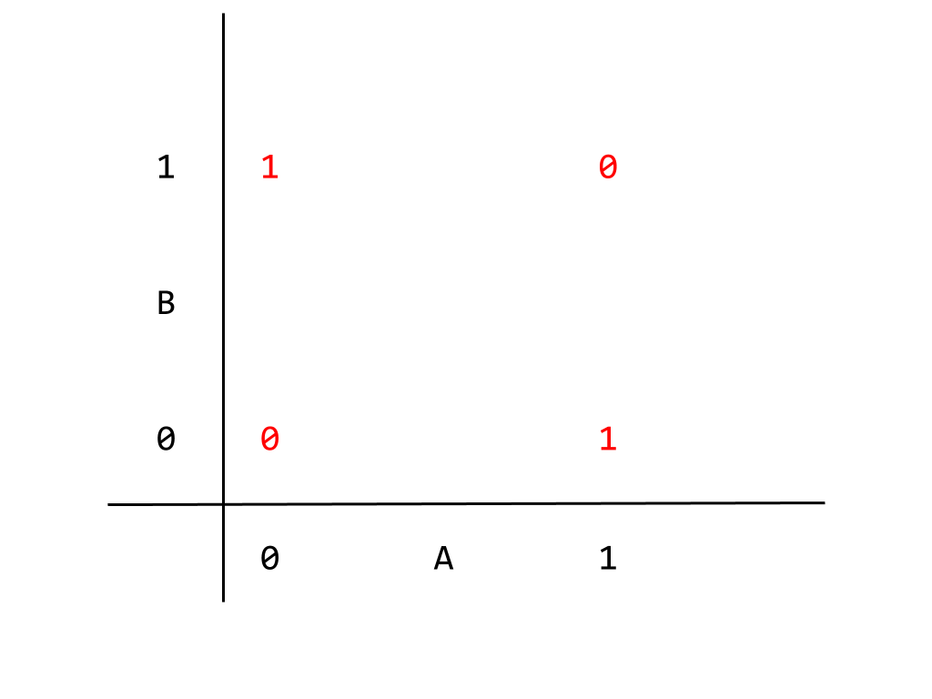
You should be able to eyeball it: we cannot find a single linear dividing boundary between the 0 and 1 outputs.
Moving on from this result, we need to add something else to our network to make it work for an XOR gate: we need to introduce nonlinear behaviour. We need to start by adding other layers of nodes between the input and output layers. This is known as a hidden layer, and is used to create intermediate correlations from our input nodes. In this context, correlation simply means some combination of nodes that produces a new activation. As with other choices we’ve made for our network so far, we are going to go with the simplest choice possible. In this case, we’ll add a single hidden layer with three nodes. Our network now looks like this,
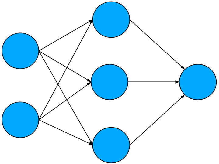
Looks great right? But this is still a linear network. To illustrate, let’s focus on one hidden layer node and the two input nodes and output node it connects to like so,
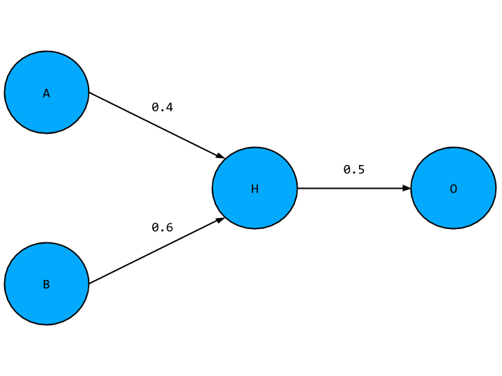
This should look familiar, with the new hidden layer node given a placeholder value H. To find the value of O in terms of A and B we first have to find the value of H. This is simply the weighted sum of A and B,
H = 0.4 * A + 0.6 * B
O is just this expression multiplied by the weight connecting H and O,
O = 0.5 * H = 0.5 * (0.4 * A + 0.6 * B)
And expanding this out,
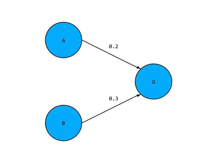
O = 0.2 * A + 0.3 * B
This looks exactly like the output we’d expect from our original linear network, which means the hidden layer node is not adding anything new to our network. In fact our hidden layer as a whole is not giving us any new correlations, so we might as well not have it in this case, and have a network with slightly tweak weights as below,
To move away from a linear network we need to add yet another component: activation functions. This is precisely so that the hidden layer activations is not just some weighted of input nodes, so our network is not simply reducible to a single input and output layer. Activation functions are just mathematical functions that determine whether a hidden layer node turns “on” or “off” for a given input. They fit within the common conceptual picture of neurons in the brain. Like our hidden layer nodes, neurons receive an electrical signal and may signal on or off if this input reaches a certain threshold. The choice of activation ultimately comes down to the kind of problem we are dealing with. The activation function we will be using is known as the “relu” function, which follows the rules:
- If the input value < 0 then return 0
- Otherwise return the original input
Turning to code we get the following,
function relu(x) {
    return iterator(x, x => ((x > 0) * x))
}

function iterator(x, fn) {
    let out = x.slice().tolist()

    for (let i = 0; i < out.length; i++) {
        for (let j = 0; j < out[i].length; j++) {
            out[i][j] = fn(out[i][j])
        }
    }

    return nj.array(out)
}
This has been refactored to use a more functional style, but the basic logic is this same. x => ((x > 0) * x) is the actual relu function as discussed, and the iterator helper function applies this element-by-element on an array of arbitrary size.
That’s a lot of material to cover already, but we now have a deep learning neural network! In the next post we will see how to run input into this network to get output and how to get the network to learn the training set data adequately.
All the best,
Tom
The Brief on Developer Book Clubs
Perhaps not much of a surprise but working as a developer requires a great need for continuous learning and growth, and of course this is not always an easy task. Some time last year, I found myself struggling to learn functional programming principles. I approached several people at work with some success, but couldn’t make the most of the opportunities for discussion - often these were just snatches of time between meetings or over a beer. Obviously there was a great willingness for learning but no real platform to make the most of it. I strongly believe that a platform and structure is perhaps the most important component when approaching a technical topic for the first time, to enable a sense of progress and reflection. This led to the creation of the developer book club at my workplace. In this blog post I want to cover how we run the club, some opinions around this point, and some general challenges we’ve faced or anticipate in the future.
How we run the book club
We have three main channels of communication: A GitHub repo, a HipChat room, and a mailing distribution list. The GitHub repo is the place where we put all the written notes and presentations, which I’ll come to later, as well as leverage the issue creation system to enable people to make reading suggestions. The HipChat room is where the majority of online discussion takes place as well as where we make general announcements and potentially vote on the next reading if this has not already been decided during the book club session. Finally, the mailing distribution list allows us to make announcements and book meeting rooms without spamming everyone.
We try to book a session every two weeks, for one hour during lunch, which has so far worked for us. When deciding on readings to focus on, we ideally want something that is freely available electronically with exercises, so that the barrier to entry is as low as possible. We tend to stick to two basic formats, the choice between them following from the kind of reading being covered. For less technical readings, we use as retrospective style format using the labels “liked”, “learned”, “lacked”, which for obvious reasons lends itself to a learning exercises. For technical readings, we use a presentation-style format: Ahead of the session, people are given a section or chapter to focus on, with the expectation that they are able to give a brief presentation in sufficient detail to cover the material. We often combine formats: our first session for a more technical reading follows a retrospective style, then once we’ve established a baseline for what everyone wants to take away from the reading, switch to a presentation style format in future sessions. In all cases, we keep some informal minutes to make note of the key talking points covered.
Going back to the example of learning functional programming, we were able to select an appropriate reading as a group, which in this case was the “Mostly Adequate Guide to Functional Programming”. We have an initial session following a retrospective format, and had two more sessions using the presentational style format. Rather than trying to make notes of everything I had trouble with whilst I read it individually or hoping to simply tease out some meaning from the text, we were able to work through individual problems we had as a group and made great progress.
I think sticking to a format is absolutely key to making the most of these sessions. Firstly, keeping written records of the sessions allows for future reference and reflection. Secondly, both formats makes sure that everyone has to talk about the reading where they may otherwise be unwilling to open up in simple freeform discussion. Finally, a more obscure point, having a format and keeping notes allows people who are unable to commit to every book club to still get involved. Even if they cannot make a session, someone can still go to the repo with an expectation for the kind and quality of notes there. More broadly, every topic we cover is much bigger than any one reading, so enabling someone who may not be able to finish the reading in time to still get involved, but may otherwise know about the topic, is very rewarding for everyone else.
A criticism of this approach might be that it stifles discussion, which is true to a certain extent, but this is also kind of the point! I feel freeform discussion is a much less effective approach to learning in general, and for the reasons above not as inclusive or enabling as a more strict format provides. Discussion will happen regardless and will be more targeted and focused overall.
Problems
That’s all well and good but what kind of problems have we faced, and what do we anticipate? The problems we’ve faced so far are all the ones you’d anticipate: how do we keep numbers up and keep a diversity of interest. We’ve done ok as far a numbers go, averaging around 5 people per session, which considering the level of commitment required is promising. However, they tend to be the same people, which could indicate we need to think more broadly when it comes to reading choices overall. A problem we anticipate in the future is how to approach much longer and more technical readings, in particular several weeks ago someone stated their interest in learning Haskell, which is obviously a big ask. Our thought would be to interlace this activity with shorter, less technical choices, so we both get good progress with the longer term goal as well as a nice turnover of topics and discussion, sessions to session.
Conclusion
Overall I think developer book clubs are a great asset to the workplace and a really important learning platform. In particular I think sticking to a strict format as much as possible makes the most of everyone’s time and makes for a greater learning experience overall.
On a more personal note, I’ve thoroughly enjoyed the time since starting the book club. Whilst I haven’t necessarily touch on topics I wouldn’t have otherwise, I have approach them in a much different way and taken a lot more away from each reading. If nothing else, it’s very enlightening to see how different people with very different skills sets approach the same material and what unique challenges they may be faced with.
In Defence of BEM
BEM is an easy target for criticism in the world of front-end development, it can be verbose, complicated, and just plain ugly. In a world of preprocessors and source maps, it is all the more important to restate some of the advantages BEM can bring,
- There is a one-to-one relationship with named selectors in stylesheets and selectors found in the DOM,
- Grepping your stylesheets is that much easier because of strict “double underscore,” “double hyphen” syntax,
- Natural extension of the above two points: no ambiguity of relationship between selectors, no need to infer by context
Let’s look at an example, the following code is adapted from Robin Rendle’s BEM 101,
.menu {
  background: #0B2027;
  &.trigger {
    background: #16414f;
    float: left;
    padding: 1.3rem 0;
    width: 10%;
    text-align: center;
    color: white;
    font-size: 1.5rem;
    -webkit-transition: .3s;
            transition: .3s;
    &.active {
      background: salmon;
    }
  }
}
Taking advantage of a preprocessor, we can nest sibling selectors to create a concise code snippet. However we can already see some possible problems that may arise,
- It is only clear what we should expect
.activeto do by reference to its nesting, we’d need to take advantage of@importrules to properly namespace, - Is this really scalable? How often can we expect this set of class names to occur in the future?
- What about JS hooks?
A fully BEM solution would produce,
.menu {
  background: #0B2027;
}

.menu__trigger {
  background: #16414f;
  float: left;
  padding: 1.3rem 0;
  width: 10%;
  text-align: center;
  color: white;
  font-size: 1.5rem;
  -webkit-transition: .3s;
          transition: .3s;
}

.menu__trigger--active {
  background: salmon;
}
Though perhaps arguably less attractive to look at, there is certainly something to said for being explicit. To slightly abuse the conclusions made in Ben Frain’s Enduring CSS, for the small risk of extra bloat in the short term, there is the promise of greater mobility in the long term. CSS selector naming is first and foremost about communicating intent to other developers, especially those that may not be exclusively front-endians. With BEM, there is an explicit flat relationship between selectors, which is clearly communicated in CSS and HTML: No need to dig around to know that .menu__trigger--active implies a state change and relates to a specific child/component.
All the best,
Tom
Serving Up Hamburger Menus - or Not
Hamburger menus have a problem. Best put by Luis Abreu’s post against needless use of the UI, hamburger menus,
- Lazily put together too many UI elements, which means that,
- They are less usable, which leads to,
- Poorer user engagement.
More important still is to remember why a hamburger menu is a popular choice for dealing with navigation in the first place: We want to transplant a desktop experience to a mobile experience. This is a crucial mistake to make, and overlooks the golden rule “content is king.” Jonathan Fielding took this head on in a recent Front-end London talk, by selectively choosing which content to prioritise for a given device. In a move towards a responsive, mobile-first web experience we are routinely required to tweak performance for efficient delivery of assets by device type. This is exactly how navigation and UI should be treated.
Instead of lumping all UI elements under the hamburger, Luis Abreu shows exactly how to keep as much up front as possible using a tab bar. This may require trimming away of some elements, or a least a tidy up a desktop navigation. Although this solution may not be entirely scalable, it at the very least allows us to engage our information architecture head-on - something that would be easily hidden by using a hamburger menu as a first step.
All the best,
Tom
Nesting Lists
Dealing with nested lists in HTML gave me pause for thought recently as though simple the markup is not immediately obvious. Intuitively I’d go for placing the markup for the nested list as a direct child of the parent list, like so,
<ul>
    <li>List item one</li>
    <li>List item two</li>
    <ul>
        <li>Subitem 1</li>
        <li>Subitem 2</li>
    </ul>
    <li>List item three</li>
</ul>
However, ul elements may only contain list item elements. Direct from the W3C wiki, “the nested list should relate to one specific list item.” Hence the markup should be,
<ul>
    <li>List item one</li>
    <li>List item two
      <ul>
          <li>Subitem 1</li>
          <li>Subitem 2</li>
      </ul>
    </li>
    <li>List item three</li>
</ul>
Minor point perhaps, but good markup is better for your users and makes your life easier in the long run.
All the best,
Tom
CSS Percentage Margin/Padding Properties
Definitely a candidate for one of my more recent WTF moments. I recently discovered, and subsequently had to work around, the following CSS behaviour: margin/padding-top/bottom percentages are calculated by reference to the width of the containing block, not the height.
This is at the very least slightly confusion especially as CSS enables you to calculate top/bottom with respect to height as expected. I’ve not found an especially clear explanation for this, however most opinions converge on the following,
- We tend to set/deal with widths, not heights explicitly,
- It makes rendering that much easier for “horizontal flow,” as discussed here,
- There has to be some shared reference between
margin-top,margin-leftetc. as settingmargin:5%is a thing.
The end result being that setting resizeable aspect ratios are a breeze as we have constant referring to the width of the element in question. Others, much braver than myself, have looked in to how to explicitly set something equivalent to top/bottom-margin. However, I would advise against this as it exploits the quirks of the CSS specification, which is never a good place to be.
All the best,
Tom
CSS Counters
CSS counters provide a really convenient way of adding academic-style numbering to your markup, with the added advantages of being well supported and easily expandable to an arbitrary indexing style and depth of nesting.
Provide you have some markup to get started on, you will need to specify the following properties counter-reset, counter-increment, and content. The first property relates to the containing element of our counters, creating a new instance for the counters. The latter two relate to how the counters are displayed on the page. For instance,
<body>
  <!-- 'Ere be imaginary markup -->
  <section class="content-section">
    <h2 class="content-section-heading">Awesome Heading</h2>
    <p class="content-text">Awesome text</p>
    <p class="content-text">Awesomer text</p>
  </section>

  <section class="content-section">
    <h2 class="content-section-heading">Another Heading</h2>
    <p class="content-text">More text</p>
  </section>

</body>
For this example, I’d like to have the elements with class “content-section-heading” numbered as “1.”, “2.”, and so forth, and each paragraph element with class “content-text” numbered as “1.1”, “1.2” etc. where the first number corresponds to the “content-section-heading”, and the second corresponds to the number of the p element. In the following we refer to the two numbers as “section”.”sub-section”,
body {
  /* Set section counter to zero */
  counter-reset: section;
}

.content-section-heading {
  /* Set sub-section counter to zero, following each "h2.content-section-heading" */
  counter-reset: sub-section;
}

.content-section-heading:before{
  /* Render section counter to page with decimal and trailing space */
  counter-increment: section;
  content: counter(section) ". ";
}

content-text:before{
  /* Render section and sub-section counter to page with decimal and trailing space */
  counter-increment: sub-section;
  content: counter(section) "." counter(sub-section) " ";
}
Altogether we should get,
<body>
  <!-- 'Ere be imaginary markup -->
  <section class="content-section">
    <h2 class="content-section-heading">1. Awesome Heading</h2>
    <p class="content-text">1.1 Awesome text</p>
    <p class="content-text">1.2 Awesomer text</p>
  </section>

  <section class="content-section">
    <h2 class="content-section-heading">2. Another Heading</h2>
    <p class="content-text">2.1 More text</p>
  </section>

</body>
CSS counters are highly customisable, allowing you to specify the unit to increment/decrement the counters, and the number of counters changed at any one time.
All the best,
Tom
JavaScript: Expressions v Statements
JavaScript, like many other languages, distinguishes between expressions and statements, which means you should too. However, the terms do not refer to a particularly clear cut syntactic difference in many cases and often the difference is largely context specific.
The simplest definition of these terms: Expressions produce a value, or stand in wherever a value is expected, these act without producing any side effects. For instance, examples are taken from Rauschmayer’s review of the subject,
myvar
3 + x
myfunc("a", "b")
On the other hand, a statement provides an action or behaviour, such as a loop, if statement, or function declaration. (Most authors lump together declarations with statements. this is not exactly true as, for instance, declarations are treated differently in the hoisting process.) An important unidirectional relationship exists between expressions and statements: A statement may always be replaced by an expression, called an expression statement. The reverse is not true. The distinction becomes more muddy from here!
A particular problem relates to the difference between function expressions and function declarations, which look essentially the same,
// Function expression
var greeting = function () { console.log("Hello!"); };

// Function declaration
function greeting() { console.log("Hello!"); };
I wasn’t lying! The devil is in the details: the function expression returns a function object which we’ve assigned to the variable greeting. The function expression here is actually anonymous - there is no name given on the right hand side of the equals sign. A named function expression such as,
// Named function expression
var greeting = function howdy() { console.log("Hello!"); };
has the name howdy that is scoped to the function expression. The function declaration on the other hand, declares a new variable, with a new function object assigned to it. This produces something equivalent to the function expression above,
var greeting = function () {
  console.log("Hello!");
};
Unlike function expressions, function declarations cannot be anonymous, which is why the the first example function expression was an expression not a declaration. This is an important point as this implies IIFE pattern has to be a function expression.
Without going into any great detail, the distinction between function expressions and function declarations also shows up again in the topic of hoisting: only function declarations are completely hoisted.
The discussion only continues from here: Whether statements or expressions are more performant - I accept it’s a nonce word, or which better lends itself to best-practices.
All the best,
Tom